ROI Estimator example for the real estate business

The estimator includes 4 main sheets to start with:

1. Lists – this sheet holds drop down lists and backend functions to support the dashboard.
2. Dashboard – this sheet will summarize all the data from your ROI projects.
3. Master sheet – this sheet is your template for a ROI project.
4. Costs Estimation – this sheet holds predetermined costs you can use to speed things up.

Let’s dive in to each sheet’s functionality.

Lists sheet

Column A:E are built to support the dashboard layout. This part will build the list of sheets that need to be included in the dashboard. To achieve this we need to follow a few simple steps:

Setup a named range for all sheets. We do this by accessing the name manager and clicking on new name:

Next let’s create a named range and add this function to it’s value. In my case SheetNames :

=REPLACE(GET.WORKBOOK(1),1,FIND(“]”,GET.WORKBOOK(1)),””)

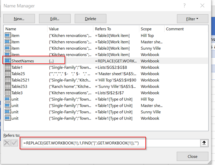
Next we build the list of sheets using this function:

=IFERROR(INDEX(SheetNames,A2),””) , where A2 is a number from 1 .

This will populate all the sheets in your file.

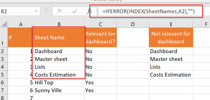
Last step is to add a list of sheets to be excluded from the dashboard. I used this function:

=IF(LEN(B2)>0,IF(ISERROR(MATCH(B2,E:E,0)),”Yes”,”No”),””)

Any sheet name you list in column E will not appear in the dashboard.

Examples of the drop-down lists for the input:

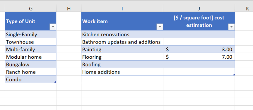
For the real estate example, I used type of housing unit and type of work item to be done. These can be easily setup for your needs. I also added a cost per square foot here for the cost estimation.

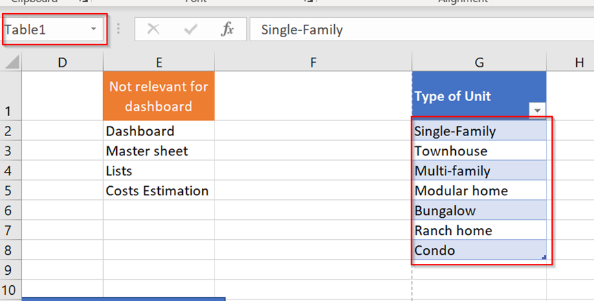
There are two tables, one for each drop down list. I assign a name to the range of the values and will use that range in the other sheets.

To do that, you need to select the cells and change the name range (where it says Table1 to unit or something else:

Cost estimation sheet

In this case I want to be able to assign a fixed value as a reference for the cost.

I built a matrix of work items and housing units. Both lists are pulled from the lists sheet automatically using array functions – unique and transpose.

The function to populate the items is =UNIQUE(Table3[[#All],[Work item]]) for the work items. =TRANSPOSE(UNIQUE(Table1[Type of Unit])) for the housing units. Any change in the lists sheets will automatically update this matrix.

For each combination I assigned a value (if available) or left empty if the cost is per square meter. For those cases the cost is pulled from the lists sheet.

Master sheet

The master sheet is your template for generating new sheets. Each project is a new sheet and will be duplicated from the master sheet after clicking on the add project button.

You need to setup the master sheet before starting so that your projects are ready to be filled. In this example there are blue columns – data to be added and orange columns – formulas.

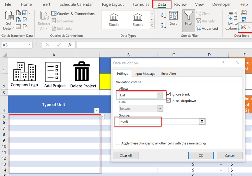
The type of unit and work item are drop down lists based the lists sheet. In order to build the drop down lists select the entire column of the table a5:a90 in this case. Then click on data, data validation, change the allow input to List and the source input to your named range. In this case =unit.

I have setup different columns for estimating the cost. The cost estimation $/square foot is a vlookup formula to the lists table. =IFERROR(VLOOKUP([@[Work Item]],Table3,2,0),0)

The fixed cost estimation is based on the sheet cost estimation and is an Index + match function. =IFERROR(INDEX(‘Costs Estimation’!$A$2:$ZZ$999,MATCH([@[Work Item]],’Costs Estimation’!$A$2:$A$999,0),MATCH([@[Type of Unit]],’Costs Estimation’!$A$2:$ZZ$2,0)),0)

Cost estimation will show the fixed amount if >0 or calculate the cost per square foot.

Another column I added is an estimation override where if you input something that will be the cost per that line.

Total project cost sums the cost estimation column and the ROI is calculated based on the future revenue and the cost.

VBA Part!!!

Add a project button – this code does the following:

1. Duplicates the master sheet.
2. Asks the user for the project name – this will also change the sheet name.
3. Force Excel to recalculate the formula.

VBA code:

Public Sub new_project()

Application.DisplayAlerts = False ‘Ignore messages during duplication

Sheets(“Master sheet”).Copy after:=Sheets(Sheets.Count) ‘Duplicate sheet

Dim NewName As String

NewName = InputBox(“What Do you Want to Name the Project ?”) ‘Ask the user for the new project name

ActiveSheet.Range(“B2”).Value = NewName ‘Input the name in the sheet

ActiveSheet.Name = NewName ‘Assign the new name to the sheet

Application.CalculateFullRebuild ‘Force excel to rebuild functions, needed for the dashboard

Application.DisplayAlerts = True ‘Stop ignoring messages

End Sub

Delete project button – this code does the following:

1. Asks the user if they are sure they want to delete the project.
2. Delete the sheet / stop the code.
3. Force Excel to recalculate the formula.

Public Sub delete_project()

Application.DisplayAlerts = False

If MsgBox(“Are you sure you want to delete this project?”, vbYesNo) = vbNo Then Exit Sub ‘Allow the user to validate deleting this project

If (ActiveSheet.Name = “Master sheet”) Then Exit Sub ‘Cant delete master sheet

ActiveSheet.Delete

Sheets(“Master sheet”).Activate

Application.DisplayAlerts = True

Application.CalculateFullRebuild

End Sub

Hidden code!

I also added a backend code that changes the sheet name when you change the cell ‘Project name’ :

Private Sub Worksheet_SelectionChange(ByVal Target As Range)

On Error Resume Next

Set Target = Range(“B2”)

Application.ActiveSheet.Name = Target

Application.CalculateFullRebuild

On Error GoTo 0

End Sub

Dashboard sheet

This sheet is fully automatic, it will populate the sheets you have in the file. Excluding the ones listed in the lists sheet. For each sheet the top line data is showing and allow you to analyse your projects.

List of sheet is pulled using the filter function:

=FILTER(Lists!B:B,Lists!C:C=”Yes”)

Pulling the data is achieved by a few nested functions:

=IF(LEN($A2)>0,OFFSET(INDIRECT(“‘”&$A2&”‘!B2″),,COLUMN()-1,,),””)

Using indirect and the sheet name I can dynamically reference a sheet.

Then using offset and the column number, I will pull the needed data for each column without changing the formula.

Expense Splitter