Grade Estimator excel file for your class tracking
I want to share with you a template for building a gradebook for your class / course.
This template can be used to track your students’ grades. You can use this file for many courses.
If you would like learn how to build this on your own stick around!

The file includes 3 sheets:
- List – information for drop down lists.
- Students – names of the students.
- Grade Tracking – the main sheet where you input the students’ grades.
Let’s dive in to each sheet’s functionality.
Lists sheet
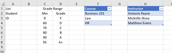
The sheet includes 4 parts:
- Column A will be used to switch between the student names and their ID. This will be used for privacy reasons.
- Grade Range – here you can group grades into letters.
- Course – you can list course names that will be used as a drop down list.
- Instructor – you can list instructor names that will be used as a drop down list
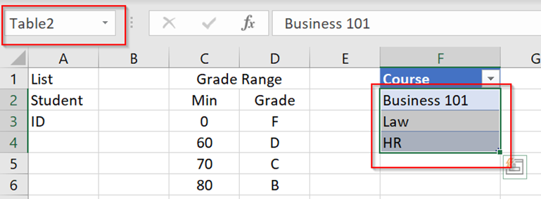
Setting up the drop down lists is done by selecting the values of the table and changing the name of the range (where is says Table 2 change to the name of the range)
Students sheet
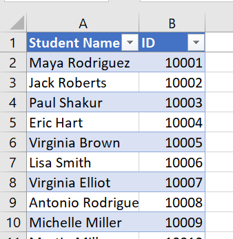
Currently the table is very simple, student name and ID. You can add more layers to this table for filtering and other options.
I named the student name range as student (like in the list sheet) and the ID numbers as ID (like in the list sheet). By using a table adding rows will automatically appear in the ranges.
Grade Tracking sheet
There are two parts for this sheet:
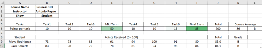
- Setting up the course details – select the course name (B1), course instructor (B2).
For each course setup the breakdown of the final grade – tasks, home work, exams etc. Each part should be assigned a number (line 6). Best to add columns between B and J so that the other formulas will not break.
- Filling in the points for each student during the course. The student names will appear in column A. They are pulled automatically from the students sheet. You need to fill in the points under each column and you will see the total points and final grade.
Let’s review the different formulas here that build the final grade:
Student names / ID
In cell B3 you can select to show student or ID as the name appearing here. Once selected the names will change.
A very simple function is used to do this :
=INDIRECT(B3) , by using Indirect I am referencing the cell which holds a named range. As a results it is being populate. This is why you need to setup the list sheet.
Total grade for each student :
=IF(A9>0,SUMPRODUCT(B9:I9,$B$6:$I$6)/J$6,””)
If (a9>0 – this ensure that if this line is empty , a blank value will appear.
Sumproduct( ) – this function multiplies two arrays, in this case the points of the tasks and the grades. Finally I’m dividing this number by the total #of points for all tasks. The end result is a weighted average which is the total grade.
The final grade is a simple formula :
=IF(A9>0,VLOOKUP(J9,List!$C:$D,2,1),””) the 1 and the end of the vlookup will find the closest value descending to the value being searched.
That is how this file is built, you can duplicate the grade tracking sheet to track many courses for the same group of students.
Cheers!
Thanks