Excel Vlookup, it’s a classic and an Excel blog would not be complete without. So I will share with you my version of Vlookup in hopes to teach you something new. Basically Vlookup connects between two tables and allows you to pull data from table #2 to table #1 based on a match for a certain value.
Excel Vlookup example
For this example let’s look at table #2 :
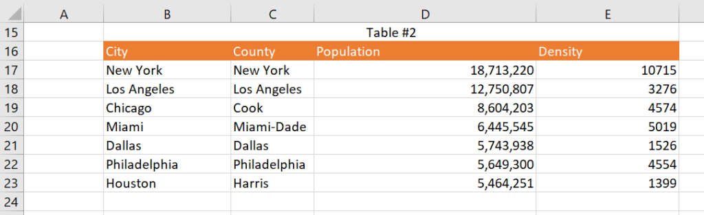
You can see the table has 4 columns, I’m going to use City as the key for the search.
In table 1 I am pulling the data from table 2 using Vlookup:
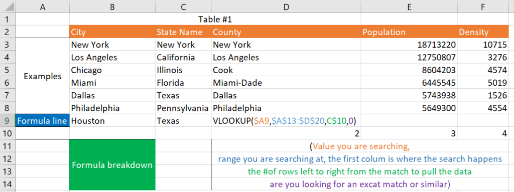
Here you see that City appears and this will be the key for the search. I want to pull the data from table 2 and add it to table 1. In the example I added county, population and density from table 1 based on a match of the city.
Excel Vlookup code breakdown for easy copying
Column D = VLOOKUP($A9,$A$13:$D$20,C$10,0)
Detailed explanation of the function Vlookup
1st argument – The value you are looking for a match
2nd argument – The range where the you are looking for a match and return value. Be aware that the search will happen on the first column of the range – in this case A. Make sure the range covers any column you want to pull data from.
3rd argument – #of columns left to right that you want to pull the data from. 1 is the minimum value and it will return the same value you are searching for.
4th argument – define if the match should be exact or closest sorted in ascending order.
Common errors while using Vlookup
If you get the result #Ref! , that means that argument #3 (# of columns left to right) is greater than the #of columns in argument #2 (the range you inputted).
If you get the result #N/A , that means that the value you are searching for (argument #1) does not exist.
Using Vlookup in Excel is a classic , but there are better functions to use. I highly recommend you try Index + Match. They are covered in the link below.